Using Fasterize
Noam Ross, Michael Sumner
2024-09-24
Source:vignettes/using-fasterize.Rmd
using-fasterize.Rmdfasterize is a high-performance replacement for the
rasterize() function in the raster
package.
Functionality is currently limited to rasterizing polygons in sf-type data frames.
Installation
Install the current version of fasterize from CRAN:
install.packages('fasterize')Install the development version of fasterize with devtools:
devtools::install_github("ecohealthalliance/fasterize")fasterize uses Rcpp and thus requires a compile toolchain to install from source. Testing (and most use) requires sf, which requires GDAL, GEOS, and PROJ to be installed on your system.
Usage
The main function, fasterize(), takes the same inputs as
raster::rasterize() but currently has fewer options and is
is limited to rasterizing polygons.
The raster raster() and plot() methods are
re-exported.
library(raster)
library(fasterize)
library(sf)
p1 <- rbind(c(-180,-20), c(-140,55), c(10, 0), c(-140,-60), c(-180,-20))
hole <- rbind(c(-150,-20), c(-100,-10), c(-110,20), c(-150,-20))
p1 <- list(p1, hole)
p2 <- list(rbind(c(-10,0), c(140,60), c(160,0), c(140,-55), c(-10,0)))
p3 <- list(rbind(c(-125,0), c(0,60), c(40,5), c(15,-45), c(-125,0)))
pols <- st_sf(value = c(1,2,3),
             geometry = st_sfc(lapply(list(p1, p2, p3), st_polygon)))
r <- raster(pols, res = 1)
r <- fasterize(pols, r, field = "value", fun="sum")
plot(r)
Performance
Let’s compare fasterize() to
raster::rasterize():
pols_r <- as(pols, "Spatial")
bench <- microbenchmark::microbenchmark(
  rasterize = r <- raster::rasterize(pols_r, r, field = "value", fun="sum"),
  fasterize = f <- fasterize(pols, r, field = "value", fun="sum"),
  unit = "ms"
)
print(bench, digits = 3)
#> Unit: milliseconds
#> expr min lq mean median uq max neval cld
#> rasterize 340.376 359.69 379.197 369.552 386.65 497.83 100 b
#> fasterize 0.337 0.37 0.545 0.414 0.64 2.51 100 aNote that even with terra, it’s still faster.
pols_v <- terra::vect(pols_r)
rt <- terra::rast(r)
bench <- microbenchmark::microbenchmark(
  terra_rasterize = r0 <- terra::rasterize(pols_v, rt, field = "value", fun="sum"),
  fasterize = f <- fasterize(pols, r, field = "value", fun="sum"),
  unit = "ms"
)
print(bench, digits = 3)
#> Unit: milliseconds
#> expr min lq mean median uq max neval cld
#> rasterize 6.148 6.939 7.66 7.22 7.45 50.5 100 b
#> fasterize 0.875 0.931 1.19 0.97 1.00 21.4 100 a We can do even better if we don’t materialize the pixel values and simply use the created index in efficient ways - but currently, we have to actually allocate the entire raster so there’s a simple memory limit there (and we’re always using double floating point type). Please see the Issues on the project respository and the CONTRIBUTING.md if you are interested.
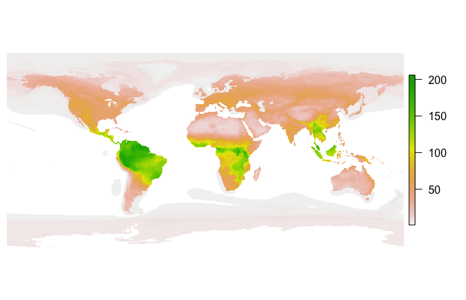
How does fasterize() do on a large set of polygons? Here
download the IUCN shapefile for the ranges of all terrestrial mammals
and generate a 1/6 degree world map of mammalian biodiversity by
rasterizing all the layers.
if(!dir.exists("Mammals_Terrestrial")) {
  download.file(
    "https://s3.amazonaws.com/hp3-shapefiles/Mammals_Terrestrial.zip",
    destfile = "Mammals_Terrestrial.zip") # <-- 383 MB
  unzip("Mammals_Terrestrial.zip", exdir = ".")
  unlink("Mammals_Terrestrial.zip")
}
mammal_shapes <- st_read("Mammals_Terrestrial")#> Reading layer `Mammals_Terrestrial' from data source `/Users/noamross/dropbox-eha/projects-eha/fasterize/Mammals_Terrestrial' using driver `ESRI Shapefile'
#> Simple feature collection with 42714 features and 27 fields
#> geometry type: MULTIPOLYGON
#> dimension: XY
#> bbox: xmin: -180 ymin: -85.58276 xmax: 180 ymax: 89.99999
#> epsg (SRID): 4326
#> proj4string: +proj=longlat +datum=WGS84 +no_defs
mammal_raster <- raster(mammal_shapes, res = 1/6)
bench2 <- microbenchmark::microbenchmark(
  mammals = mammal_raster <- fasterize(mammal_shapes, mammal_raster, fun="sum"),
  times=20, unit = "s")
print(bench2, digits=3)
#> Unit: seconds
#> expr min lq mean median uq max neval
#> mammals 0.856 0.869 0.887 0.88 0.902 0.955 20

